Example usage
Here we will demonstrate how to use pyeasyeda in a project:
Imports
import pandas as pd
from pyeasyeda.clean_up import clean_up
from pyeasyeda.birds_eye_view import birds_eye_view
from pyeasyeda.close_up import close_up
from pyeasyeda.summary_suggestions import summary_suggestions
Create dataframe
df = pd.read_csv("../tests/data/penguins_test.csv")
Clean up
This function takes a dataframe object and returns a cleaned version with rows containing any NaN values dropped. It also inspects the clean dataframe and prints a list of potential outliers for each explanatory variable, based on the threshold distance of 3 standard deviations.
clean_up(df)
**The following potenital outliers were detected:**
Variable bill_length_mm:
[600.2 700. ]
Variable bill_depth_mm:
[800.]
| species | island | bill_length_mm | bill_depth_mm | flipper_length_mm | body_mass_g | sex | year | |
|---|---|---|---|---|---|---|---|---|
| 0 | Adelie | Torgersen | 39.1 | 18.7 | 181.0 | 3750.0 | male | 2007 |
| 1 | Adelie | Torgersen | 39.5 | 17.4 | 186.0 | 3800.0 | female | 2007 |
| 2 | Adelie | Torgersen | 40.3 | 18.0 | 195.0 | 3250.0 | female | 2007 |
| 3 | Adelie | Torgersen | 36.7 | 19.3 | 193.0 | 3450.0 | female | 2007 |
| 4 | Adelie | Torgersen | 700.0 | 20.6 | 190.0 | 3650.0 | male | 2007 |
| ... | ... | ... | ... | ... | ... | ... | ... | ... |
| 328 | Chinstrap | Dream | 55.8 | 19.8 | 207.0 | 4000.0 | male | 2009 |
| 329 | Chinstrap | Dream | 43.5 | 18.1 | 202.0 | 3400.0 | female | 2009 |
| 330 | Chinstrap | Dream | 49.6 | 18.2 | 193.0 | 3775.0 | male | 2009 |
| 331 | Chinstrap | Dream | 50.8 | 19.0 | 210.0 | 4100.0 | male | 2009 |
| 332 | Chinstrap | Dream | 50.2 | 18.7 | 198.0 | 3775.0 | female | 2009 |
333 rows × 8 columns
Birds eye view
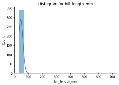
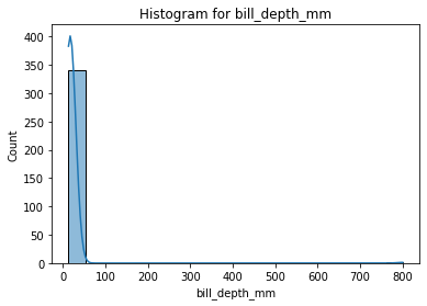
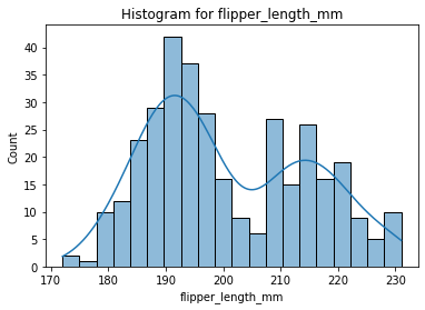
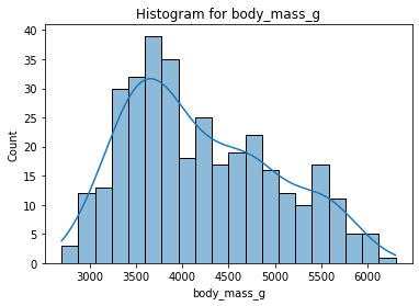
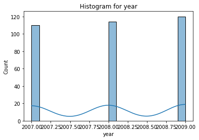
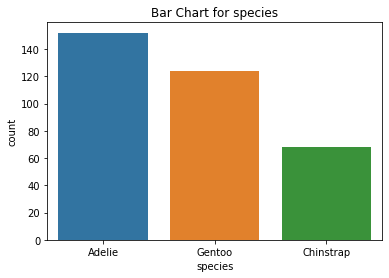
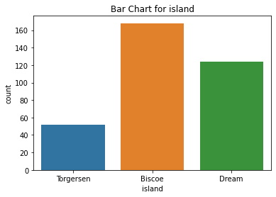
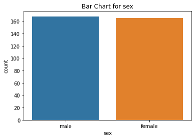
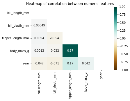
This function takes in a pandas.DataFrame object, an optional integer for the histogram bin size, an optional custom variable list, and displays 3 different visualization sets.
Histograms for each numeric variable
A bar chart for each categorical variable
A correlation heatmap of the numeric variables.
plots = birds_eye_view(df)
AxesSubplot(0.125,0.125;0.62x0.755)
<Figure size 864x432 with 0 Axes>
Close up
This function accepts a dataframe and the number of pairs of variables with strongest correlations, and returns vertically combined scatterplots with a correlation trend for each pair.
close_up(df, 1)
Summary suggestions
This function takes in a pandas dataframe and returns a list object comprising of 3 dataframes and a list. The dataframes correspond to the summary statistics of numeric and categorical variables each and the proportion of unique values for categorical variables. The nested list is of the categorical variables that exceed the threshold for considering dropping variables with high unique values.
summary_suggestions(df)
[       bill_length_mm  bill_depth_mm  flipper_length_mm  body_mass_g  \
 count      342.000000     342.000000         342.000000   342.000000
 mean        47.502924      19.427485         200.915205  4201.754386
 std         46.759549      42.377687          14.061714   801.954536
 min         32.100000      13.100000         172.000000  2700.000000
 25%         39.500000      15.600000         190.000000  3550.000000
 50%         44.500000      17.300000         197.000000  4050.000000
 75%         48.575000      18.700000         213.000000  4750.000000
 max        700.000000     800.000000         231.000000  6300.000000

               year
 count   344.000000
 mean   2008.029070
 std       0.818356
 min    2007.000000
 25%    2007.000000
 50%    2008.000000
 75%    2009.000000
 max    2009.000000  ,
        species  island   sex
 count      344     344   333
 unique       3       3     2
 top     Adelie  Biscoe  male
 freq       152     168   168,
          species    island       sex
 unique  0.008721  0.008721  0.005814,
 []]